
The needs for the solution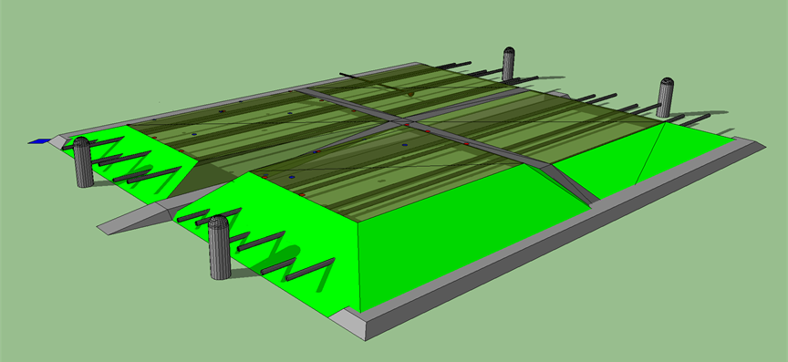
Nowadays calculation speeds
In the modern technology the large computing power is available.
The current CPU (central processor unit) processor frequency reaches up to 4 GHz. GPU (graphical processor unit) and graphics processor cards have reached up to 1,000 units in a single map, and each processor frequency reaches up to 1GHz.
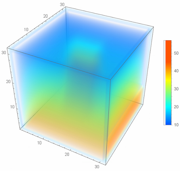
This means that it is possible to create a computer system that could be designed for solving non-stationary physical phenomena modelling problem of the three-dimensional space.
Heat conduction
The assumed initial boundary condition for the 3D domain G∪Γ is described as follows:

with the corresponding initial and boundary conditions (x1 = x, x2 = y, x3 = z) ∈ Γ, where T = temperature, t = time, x, y and z are coordinate directions, Vx, Vy, Vz = heat transferring velocity in x, y, and z directions, RT – heat retention factor and Λ12 is a heat conduction tensor, where (1) is calculable direction and (2) is a sub direction of direction 1, n = porosity coefficient of material, Q = heat source produced heat in {i,j,k} point.
Robin boundary conditions are used for this calculations.
This 3D temperature distribution equation is implemented as follows:

where T = temperature, t = time, x, y and z are coordinate directions, Vx, Vy, Vz = heat transferring velocity in x, y, and z directions, RT – heat retention factor and Λ12 is a heat conduction tensor, where (1) is calculable direction and (2) is a sub direction of direction 1, n = porosity coefficient of material.
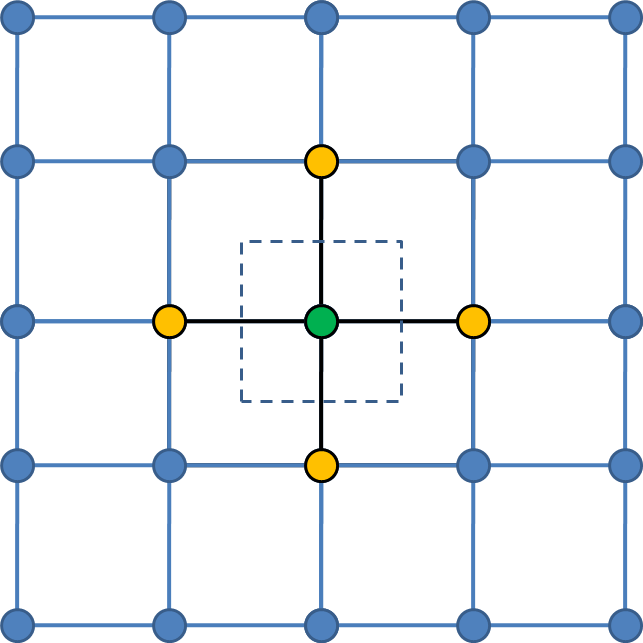
5 point stencil for every 2D
Heat conduction
We get the following differential scheme for temperature calculations from the time moment “l” to the time moment “l+1”:
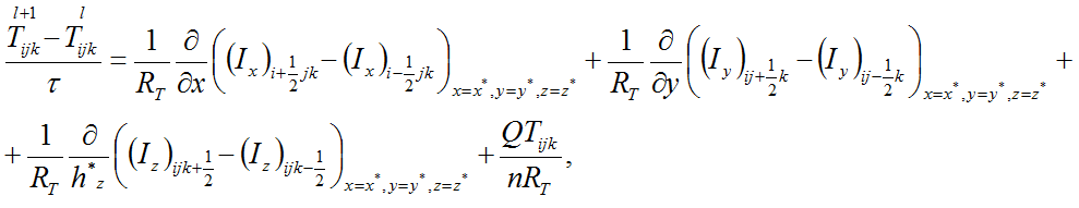
where l = current time step, l+1 next time step, i = discrete position of x, j = discrete position of y, k = discrete position of z, Q = heat source produced heat in point {i,j,k}, Tijk = temperature on the current time step in point {i,j,k}, n = porosity coefficient of material, h*x = (hx+1 + hx) / 2, where hx (step in direction of x) = xi – xi-1.
Averaged flux in x, y and z directions are expressed as follows (equations for x direction are similar to y and z direction equations):
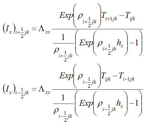
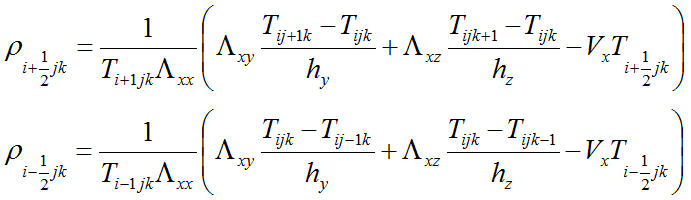
Notice that (Ix)i+1/2jk is calculated similar to other parameters’ calculations:

According to Λ the definition is (same for x, y and z axes directions):

where n = porosity coefficient of material, q = water density, c = specific heat capacity of water (it is assumed that heat source is located inside water because of assumed chemical reactions in water which produces the heat), βc,β_T= longitudinal and transverse thermo-dispersivity, and is V = the absolute velocity, vx, vy, vz = the velocity vectors.
In order to elaborate the parallel calculation method, the difference scheme was decomposed by space and time by applying ADI method:
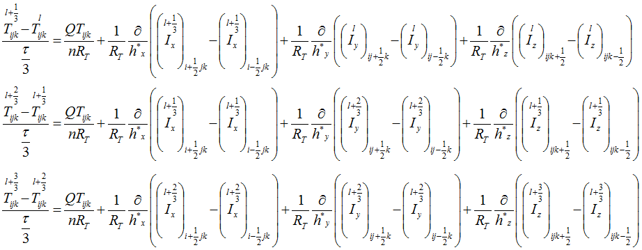
The ADI technology is used to compute calculations faster and to make implicit difference scheme, the 5 point stencil per 2 axes direction is used. So the ADI technology provides 3 diagonal matrix usage in the Thomas algorithm. Therefore, it makes very fast and efficient calculations.
The other method, for making faster calculations, it is the calculation time step that changes according to the predictions of how the temperature distribution relative to the previous time step calculation results.
Enhancements
In order to make calculation time enhancement the modified time step was created by using absolute and relative errors of calculated temperature for l+1 time moment
Absolute and relative errors calculations for X direction (same for Y and Z)
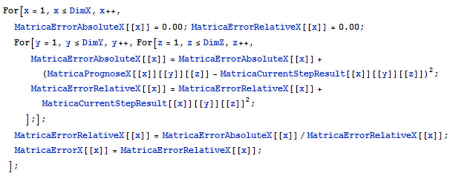
Finding the maximal error for X direction (same for Y and Z)

In order to make calculation time enhancement the modified time step was created by using absolute and relative errors of calculated temperature for l+1 time moment
Finding the next time step length:

where ErrorXYZ = maximal error between predicted and calculated results, toltol = error threshold, tau1 = temporary variable, tau = time step, taukoef = coefficient of time step changing, taumin = minimal time step, taumax = maximal time step.
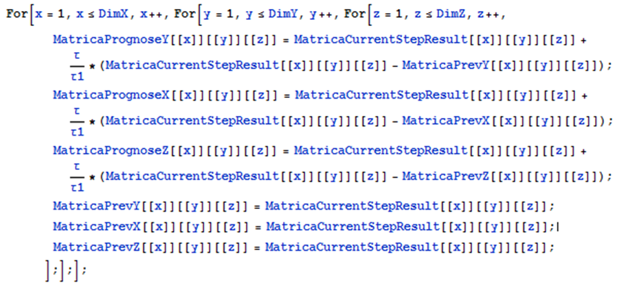
New prognoses of next time step temperature matrixes:
The solution data
Porosity: n=0,20
Solid phase density: ρs=2,2 Kg/m3
Water density at Tr: ρf=999,24 kg/m3
Specific heat cap. of water: cf=4186 J/kg.°C
Specific heat cap. of solid phase: cs=837,2 J/kg.°C
Long. Thermodispersivity: βL=10 m
Trans. Thermodispersivity: βT=1 m
Water heat capacity: ρfcf= 4183 kJ/m3.°C
Retardation coefficient: RT=2,32
Water heat conductivity: λf=0,54 J/ms°C
Solid phase heat conductivity: λs=2,09 J/ms°C
Aquifer heat conductivity: λe=1,67 J/ms°C
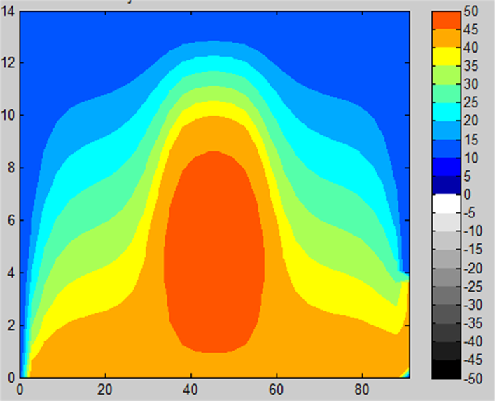
Calculation results

Outside temperature is -20 oC

Outside temperature is -10 oC

Outside temperature is 0 oC

Outside temperature is +10 oC
Outside temperature is +20 oC

Outside temperature is +14.5 oC
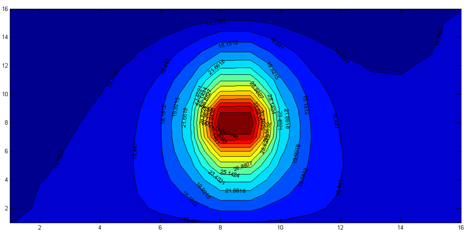
Video example of execution (y=5) from 10x10x10 matrix
Demonstration files
Just download these files and extract on drive C.
Then run this whole code fragment using MatLAB (need to replace all ‘ sings with non HTML ‘ sings or just download TempCalc.m):
clear
clc
MainDir=’C:\TempCalc’;
colorDepth = 10;
temp_max = +50;
temp_delta = +5;
temp_min = -50;
%cmap = [flipud(gray(colorDepth)); jet(colorDepth)];
cmap = [gray(colorDepth); jet(colorDepth)];
colormap(cmap);
for i=0:5:1000000
if i == 0
continue
end
fprintf(‘%s\n’,strcat(MainDir,’\’,num2str(i),’\ALL_INFO_IS_SAVED’));
while (exist(strcat(MainDir,’\’,num2str(i),’\ALL_INFO_IS_SAVED’)) == 0)
pause(1*1000*0.001)
end;
x = importdata(strcat(MainDir,’\’,num2str(i),’\DynPointsX_y16zx.txt’));
y = importdata(strcat(MainDir,’\’,num2str(i),’\DynPointsZ_y16zx.txt’));
data = importdata(strcat(MainDir,’\’,num2str(i),’\Result_y16.txt’ ));
data2 = importdata(strcat(MainDir,’\’,num2str(i),’\absolutt.txt’ ));
%[C,h] = contourf(x,y,flipud(data),[temp_min:temp_delta:temp_max]);
[C,h] = contourf(x,y,rot90(flipud(data)),10);
clabel(C,h);
hold on;
title(strcat(‘Iteracija ir:’,num2str(i),’. Laiks ir:’,num2str(data2),’sek.’));
caxis([temp_min temp_max]);
[C,h] = contourf(x,y,rot90(flipud(data)),10);
%clabel(C,h,’FontSize’,10,’Color’,’g’,’Rotation’,0);
set(h, ‘LineWidth’,1.0);
shading flat;
mycolorbar = colorbar(‘location’,’EastOutside’);
set(mycolorbar, ‘Ylim’, [temp_min temp_max]);
set(mycolorbar, ‘YTick’, temp_min:temp_delta:temp_max);
hold off;
clear x y data data2 mycolorbar;
pause(0.01*1000*0.001)
end;
clear MainDir colorDepth temp_max temp_delta temp_min cmap;