
Neuron general overview
There are 10^11 neurons in the human brain. Neurons are unique in the sense that only they can transmit electrical signals over long distances.
From the neuronal level we can go down to cell biophysics and to the molecular biology of gene regulation. In addition, from the neuronal level we can go up to neuronal circuits, to cortical structures, to the entire brain, and finally to the behavior of the organism.

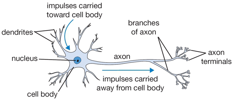
A typical neuron receives inputs from more than 10,000 other neurons through the contacts on its dendritic tree called synapses. The inputs produce electrical transmembrane currents that change the membrane potential of the neuron. Synaptic currents produce changes, called postsynaptic potentials (PSPs).
Small currents produce small PSPs; larger currents produce significant PSPs that can be amplified by the voltage-sensitive channels embedded in the neuronal membrane and lead to the generation of an action potential or spike, an abrupt and transient change of membrane voltage that propagates to other neurons via a long protrusion called an axon.


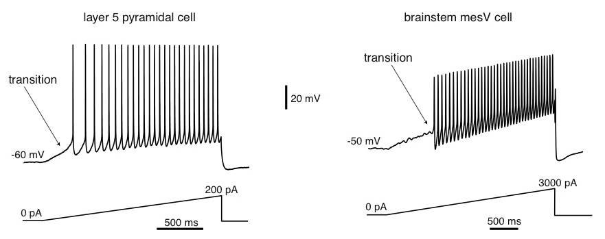
The transition between resting and spiking modes could be triggered by intrinsic slow conductances, resulting in the bursting behavior.
There could be millions of different electrophysiological mechanisms of excitability and spiking.

Ways to simulate the neuron work
There are a lot of ways to simulate the neuron work developed to make adaptive and adaptive response systems.
- Hodgkin-Huxley Model was produced by Hodgkin and Huxley in 1952. The model explains the ionic mechanisms underlying the initiation and propagation of action potentials in the squid giant axon.
- Izhikevich Model is transformed continuous-time Euler’s Discretization.
- 3 Rulkov Models can be used in different chaos prediction.
- Courbage–Nekorkin–Vdovin (CNV) Model is quite similar to chaotic Rulkov Model.
- etc.
The Izhikevich Model was chosen to be used for numerical experiment.
Alzheimer’s Disease Modeling
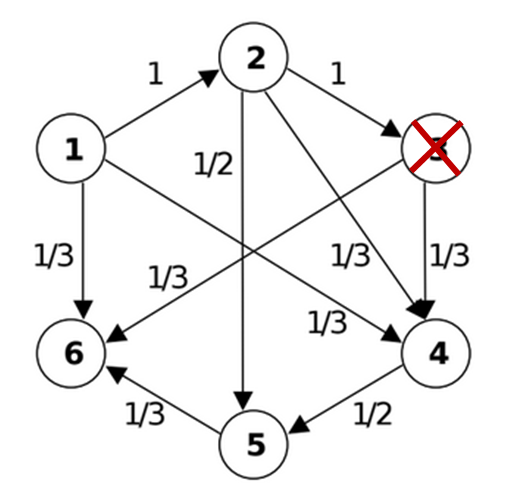
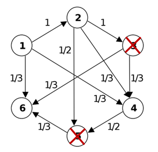
The Alzheimer’s disease problem for the brain is a fast and tending neuron isolation from the brain neural network. It means that during the Alzheimer’s disease the brain “loose” cells of memory and analytical skills developed in whole live time. Eventually, some part of neural network can loose connections to whole neuron clusters even if they produce signals between themselves.

The Izhikevich Model
The Izhikevich Model is originally continuous-time, but Euler discretization with a time step of 1 ms transforms it into the map.
There are several parameters needed for making Izhikevich neural map-based neural model calculations for calculating the membrane voltage difference between inside and outside) sides and additional variable.

- Calculable equation in Izhikevich Model:
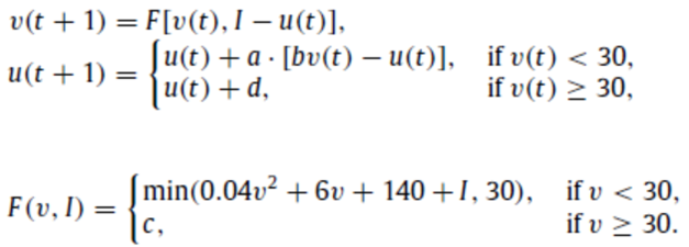
where v [mV] is membrane voltage (potential), u [mV] represents a membrane recovery variable, which accounts for the activation of K+ ionic currents and inactivation of Na+ ionic currents is additional variable depends on membrane voltage, I (synaptic currents or injected dc-currents) is electricity source connected from outside, a, b, c and d are just neuron parameters.
- Another way of these equations:

- The parameter a – describes the time scale of the recovery variable u. Smaller values result in slower recovery. A typical value is a=0,02.
- The parameter b – describes the sensitivity of the recovery variable u to the subthreshold fluctuations of the membrane potential v. Greater values couple v and u more strongly resulting in possible subthreshold oscillations and low-threshold spiking dynamics. A typical value is b=0,2.
- The parameter c – describes the after-spike reset value of the membrane potential v caused by the fast high-threshold K+ conductances. A typical value is c=-65mV.
- The parameter d – describes after-spike reset of the recovery variable u caused by slow high-threshold Na+ and K+ conductances. A typical value is d=2.
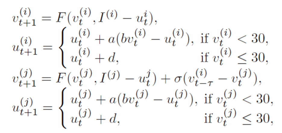
The equations for coupled neurons are:
For one of variations of the neuron parameters values the v and u plot would be these:
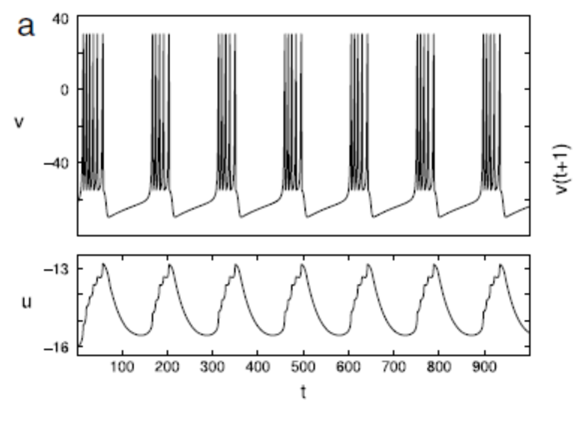
Time evolution of the Izhikevich Model variables in a bursting orbit. Parameter values are
a = 0.02, b = 0.25, c = −55, d = 0. I = 0.8.
Let’s assume there are 2 neurons without delay, so the average time distance between spikes for different v values are:
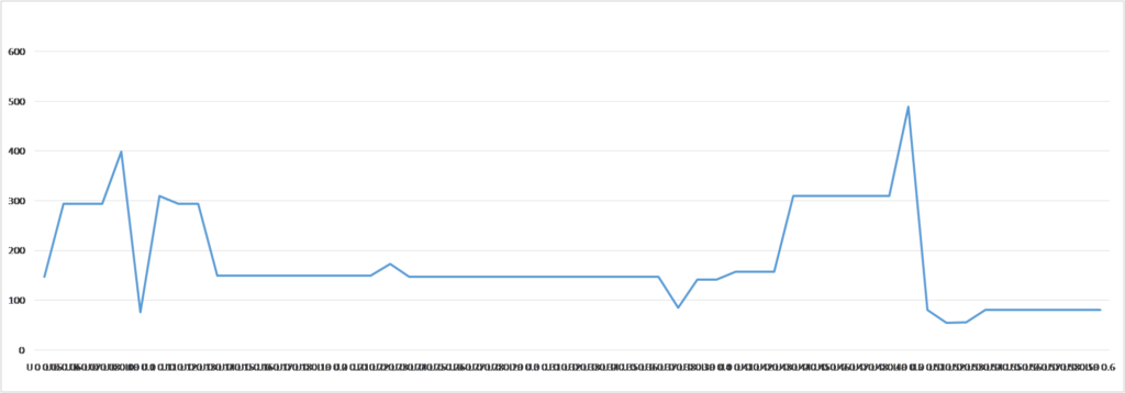
Let’s assume there are 2 neurons with 1 time moment delay, so the average time distance between spikes for different v values are:
Let’s assume there are 2 neurons with 2 time moment delay, so the average time distance between spikes for different v values are:

Let’s assume there are 2 neurons with 3 time moment delay, so the average time distance between spikes for different v values are:
Let’s assume there are 2 neurons with 3 time moment delay, so the average time distance between spikes for different v values are:
Let’s assume there are 2 neurons with 10 time moment delay, so the average time distance between spikes for different v values are:

Let’s assume there are 2 neurons with 20 time moment delay, so the average time distance between spikes for different v values are:
For numerical experiments the 6 neuron model was used implementing the connectivity matrix:

The neuron structural model is:
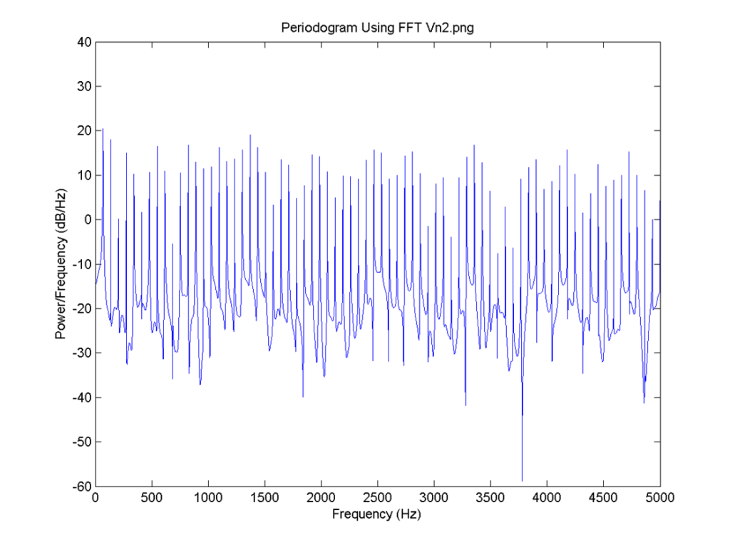
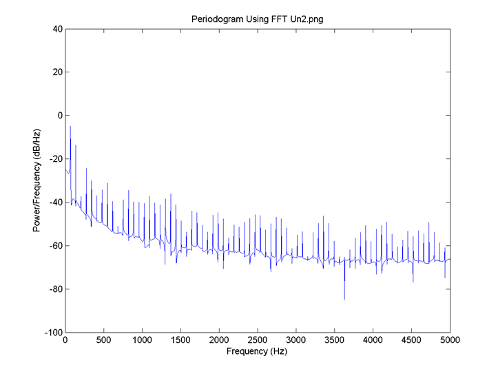
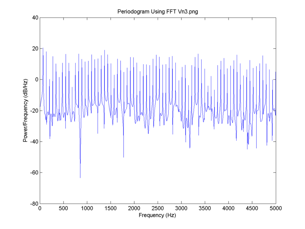
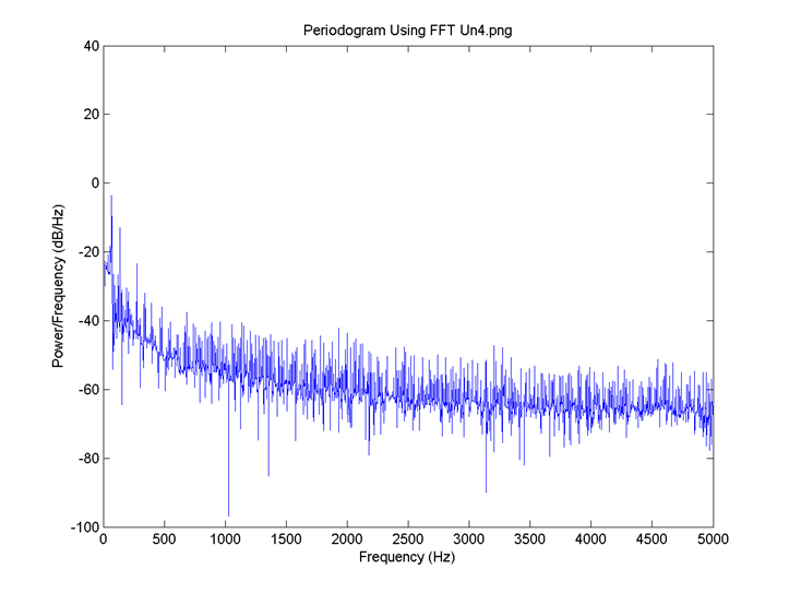
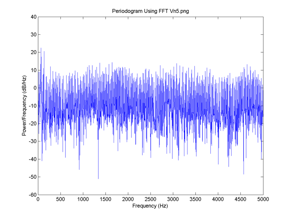
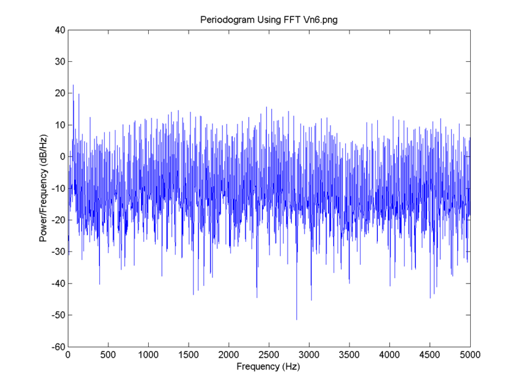
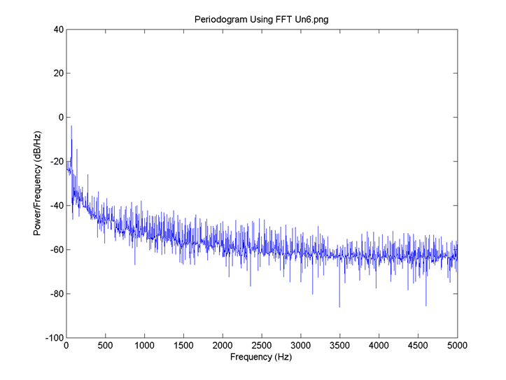
Fast Fourier Transformation allows to find calculate a kind of derivative of the equation or matrixed values approximated equation. That is why it is quite valuable to make Fourier Transformation result overview.
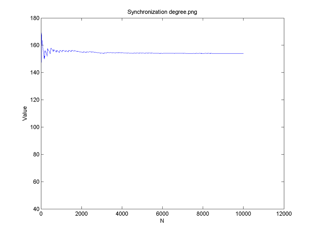
Synchronization degree, Coherence and Phase synchronization degree were analyzed for every calculation was made. And these results prove the Izhikevich Model provides the stable and periodic neuron signal model.


Numerical experiments
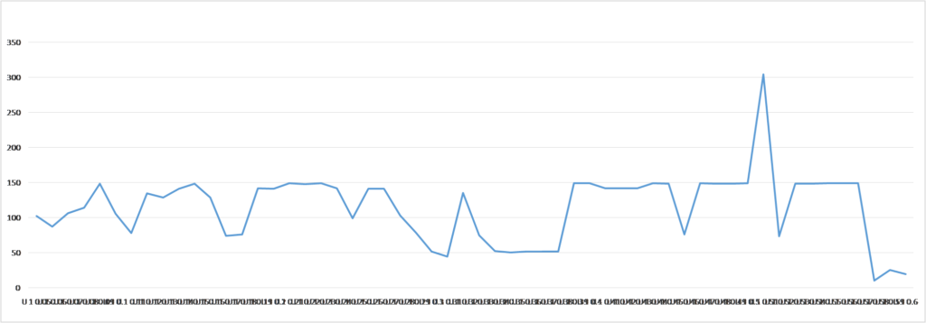
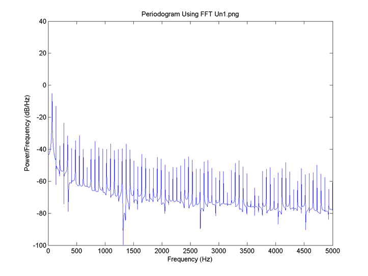
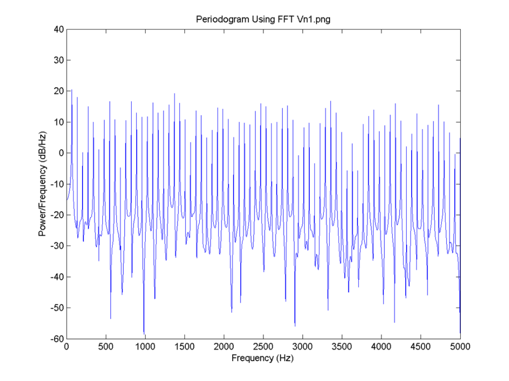
I = 0.8, there is no neuron signal delay and the connection is 0.1. FFT for 1:

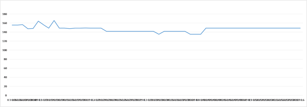
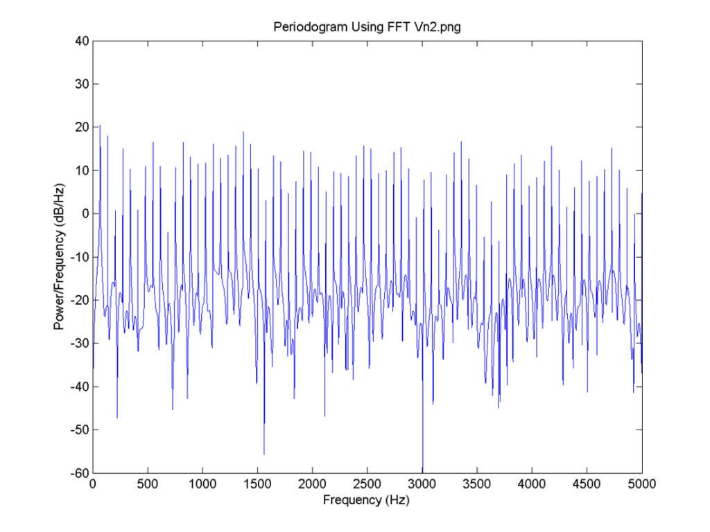
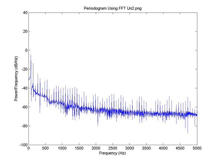
I = 0.8, there is no neuron signal delay and the connection is 0.1. FFT for 2:
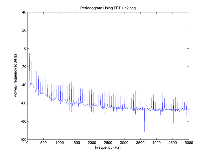
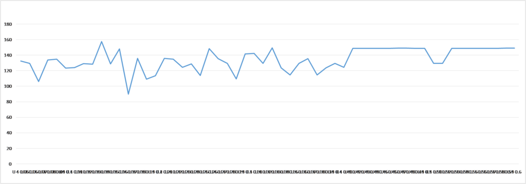
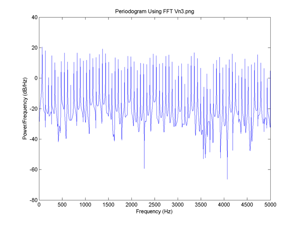
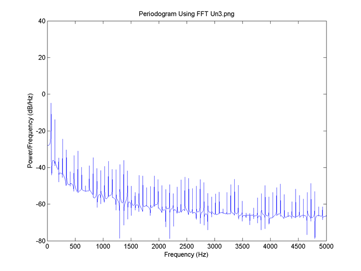
I = 0.8, there is no neuron signal delay and the connection is 0.1. FFT for 3:
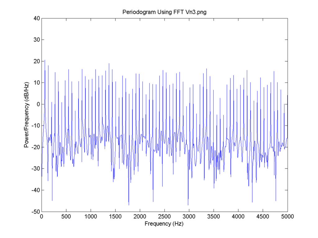

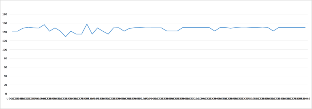
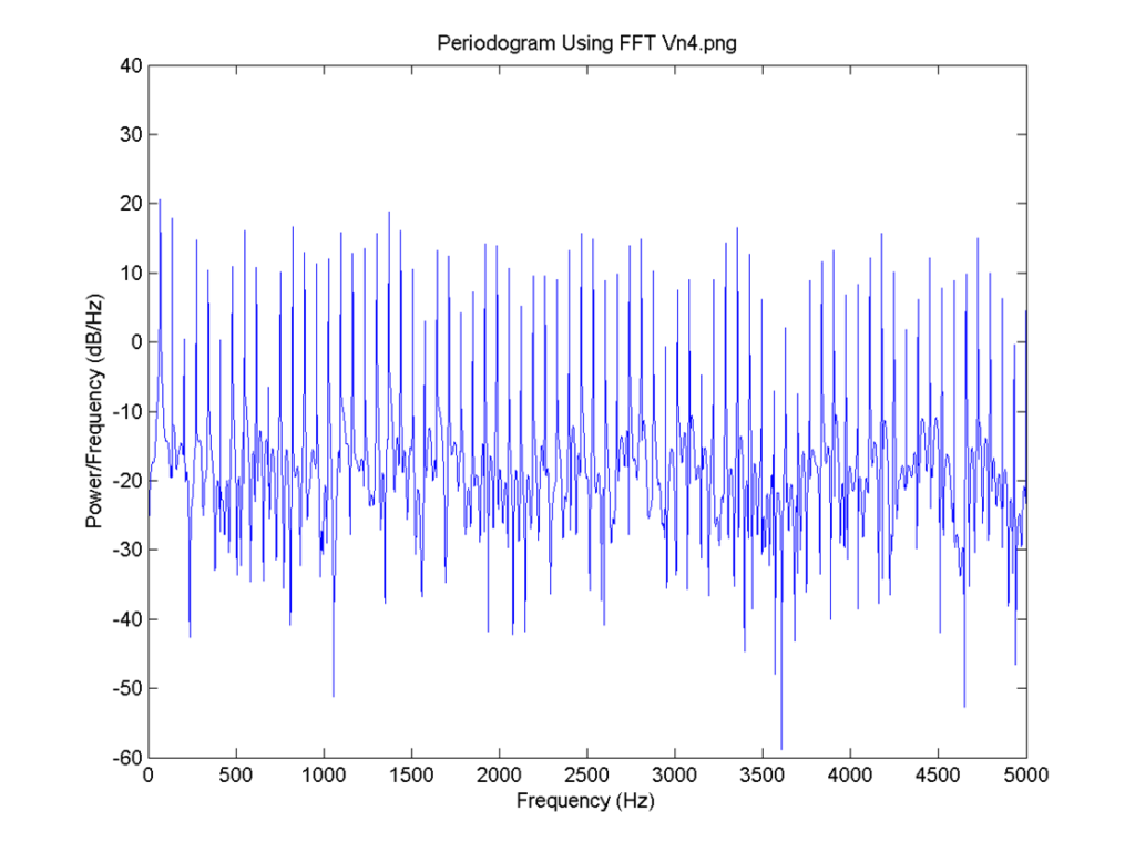
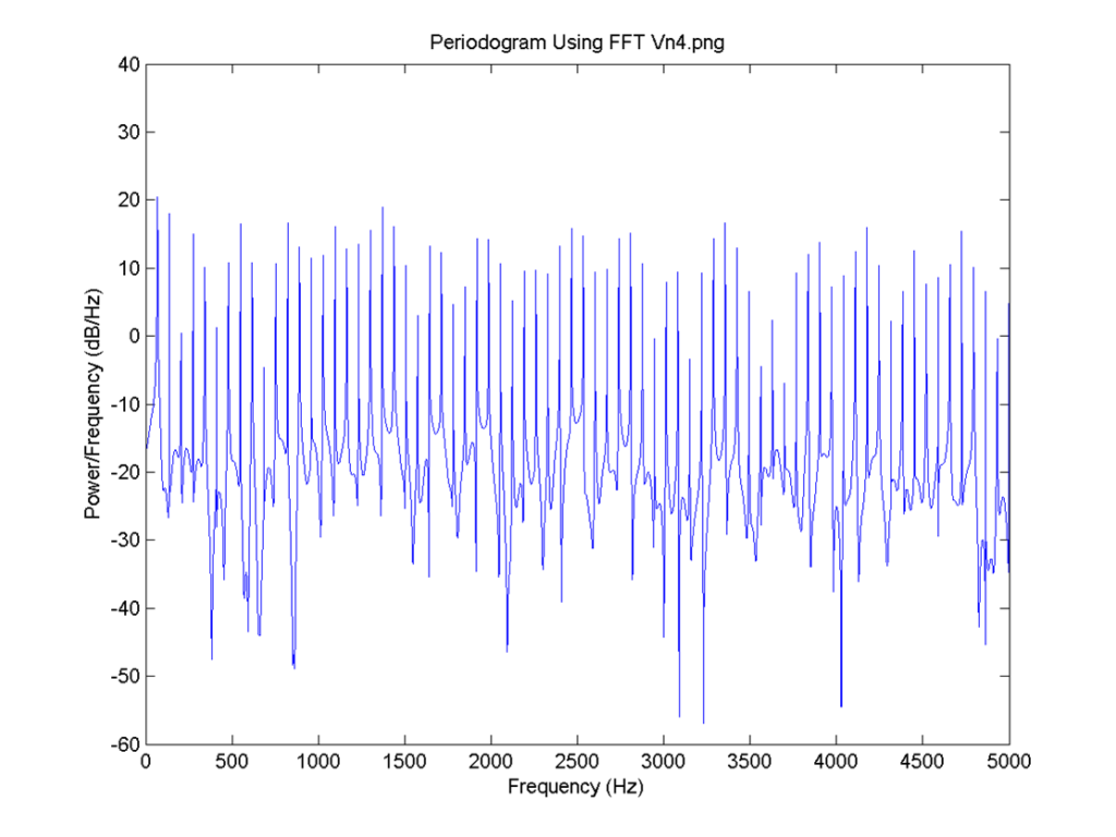
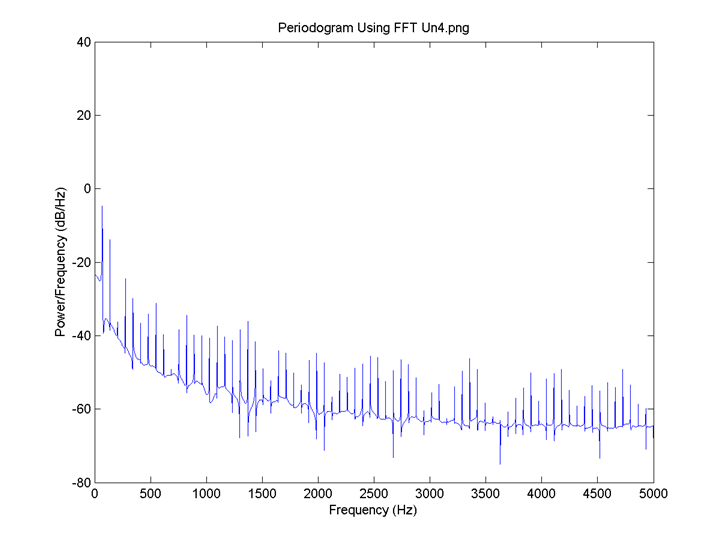
I = 0.8, the delay for all neurons is 4 time steps and the connection is 0.1. FFT for 4:

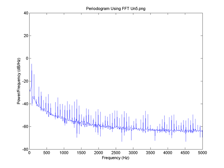
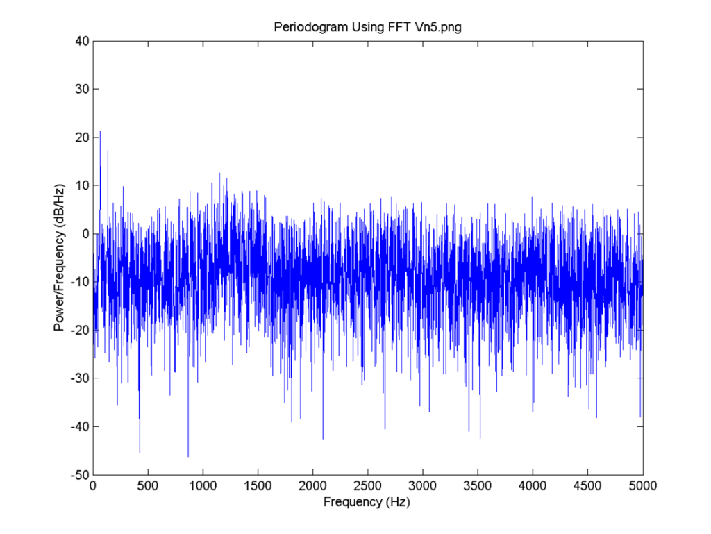
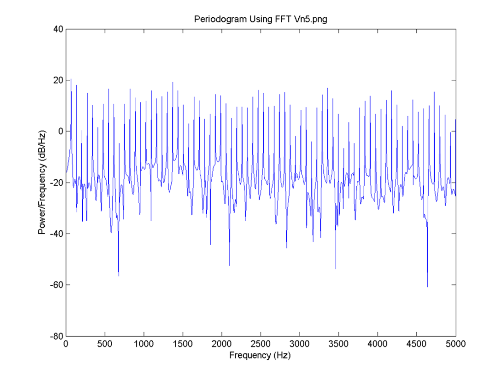
I = 0.8, there is no neuron signal delay and the connection is 0.1. FFT for 5:

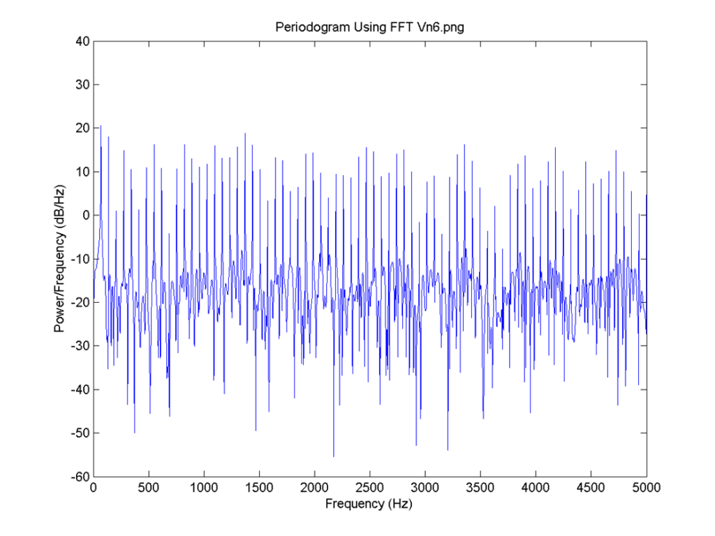
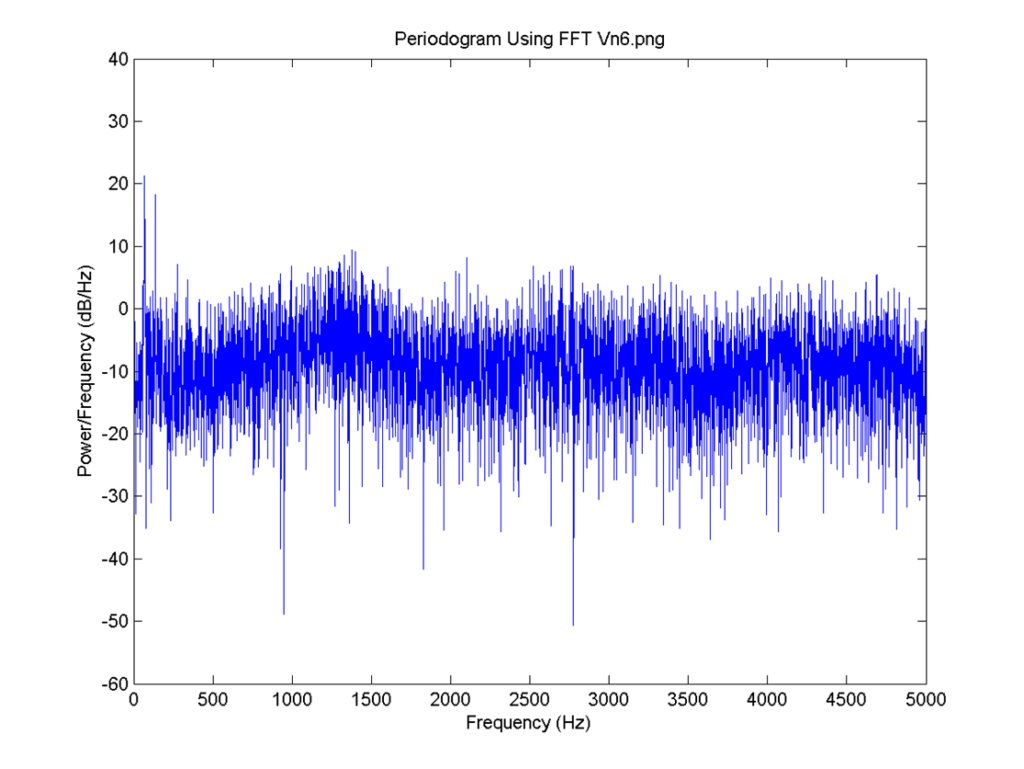
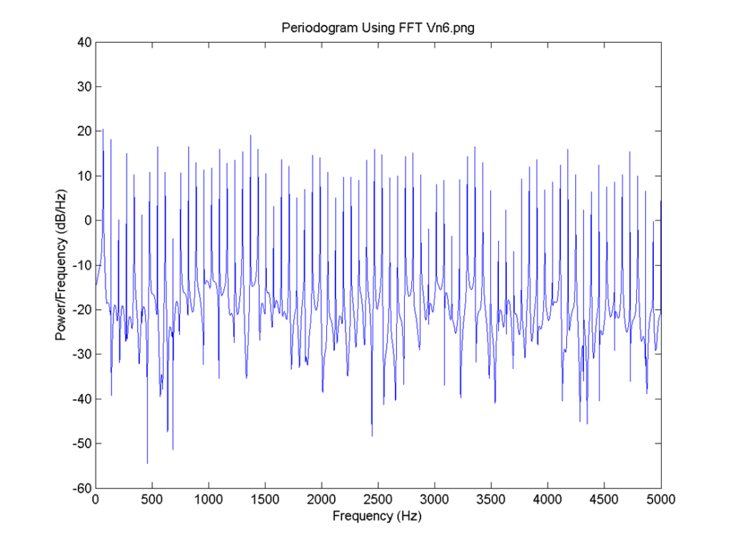
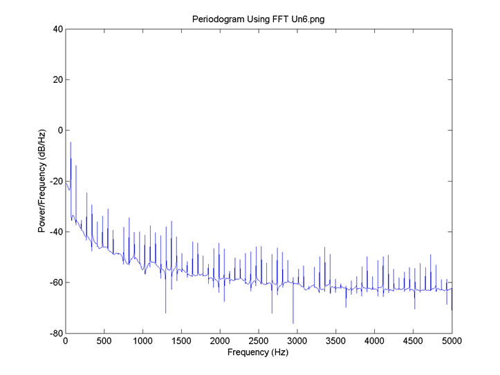
I = 0.8, there is no neuron signal delay and the connection is 0.1. FFT for 6:

I = 0.8, the delay for all neurons is 4 time steps and the connection is 0.1. FFT for 1:


I = 0.8, the delay for all neurons is 4 time steps and the connection is 0.1. FFT for 2:

I = 0.8, the delay for all neurons is 4 time steps and the connection is 0.1. FFT for 3:


I = 0.8, the delay for all neurons is 4 time steps and the connection is 0.1. FFT for 4:


I = 0.8, the delay for all neurons is 4 time steps and the connection is 0.1. FFT for 5:
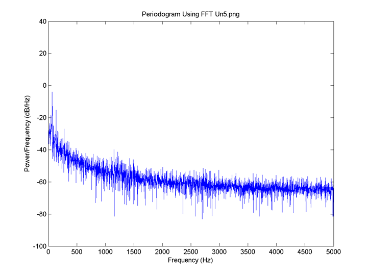
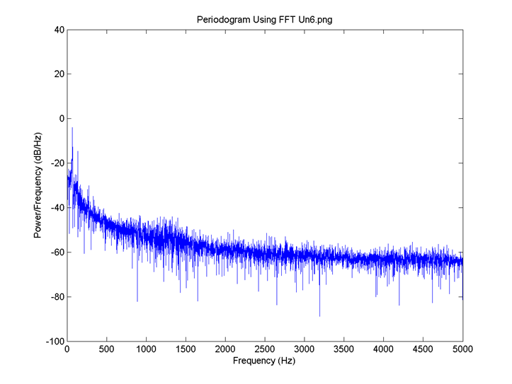
I = 0.8, the delay for all neurons is 4 time steps and the connection is 0.1. FFT for 6:
The Synchronization degree and all 6 neuron U values plot:

I = 0.8, there is no neuron signal delay and the connection is 0.6. FFT for 1:


I = 0.8, there is no neuron signal delay and the connection is 0.6. FFT for 2:
I = 0.8, there is no neuron signal delay and the connection is 0.6. FFT for 3:

I = 0.8, the delay for all neurons is 4 time steps and the connection is 0.6. FFT for 4:
I = 0.8, there is no neuron signal delay and the connection is 0.6. FFT for 5:

I = 0.8, there is no neuron signal delay and the connection is 0.6. FFT for 6:
I = 0.8, the delay for all neurons is 4 time steps and the connection is 0.6. FFT for 1:

I = 0.8, the delay for all neurons is 4 time steps and the connection is 0.6. FFT for 2:


I = 0.8, the delay for all neurons is 4 time steps and the connection is 0.6. FFT for 3:
I = 0.8, the delay for all neurons is 4 time steps and the connection is 0.6. FFT for 4:

I = 0.8, the delay for all neurons is 4 time steps and the connection is 0.6. FFT for 5:

I = 0.8, the delay for all neurons is 4 time steps and the connection is 0.6. FFT for 6:
The Synchronization degree and all 6 neuron U values plot:


Conclusions
- There are several useful neuron work simulation models.
- Several factors such as neuron signal delay and neuron isolation have to present in Alzheimer’s Disease problem analyze solutions.
- The Izhikevich Model gives stable results during calculations.
- The neuron signal receiving delay make big impact the overall neuron network system behavior.
- Neuron synchronization level impacts only the neural network stabilized state process time.